Data Science cheatsheet
General Data Science
General Terms
| Spark Term | Description |
|---|---|
| Spreadsheet | Think of data as spreadsheet |
| Statistical learning | Output = f(input) # => f(inputVariable) or f(inputVector), or f(independent variables) or Y = F(X) // X1,X2,.. |
| Programming learning | OutputAttributes = Program(InputAttributes) or Program(InputFeatures) or Model = Algorithm(Data) |
| Error | Y = f(X) + e # => You learn a function! |
| Parametric learning | No matter how much data you throw on it, it will still need these parameters like a line Y = ax + b (logistic regression, linear discriminant analysis, perceptron) |
| Non parametric learning | They fit differnet forms it’s not a single form with parameters, like Decision Trees, Naive Bayes, Support vector machines, k means. Require lot more data. |
| Supervised | You have a teacher he knows the answer, classification, regression |
| Non supervised | No teacher, clustering, association |
| Semi supervised | Some can be with a teacher |
| Bias Variance Trade Off | Bias Error (model assumptions), Variance Error, Irreducable Error. Increasing bias error reduce variance, increase variance will decrease bias |
| Avoiding overfitting | Resampling to estimate model accuracy, Hold back validation dataset, Cross validation. |
| Gradiant Descent | Optimization - almost every machine learning algorithm uses optimisation at it’s core, optimising the target function. Local minimum. start with 0 coefficient = 0.0. cost = evaluate(f(coefficient)). Update coefficient downhill with derivative. coefficient = coefficient - (alpha * delta). alpha learning parameter. |
| Stochastic Gradiant Descent | Have large amounts of data, update to coefficients is foe each training instance, not in batch, as we have random data we move quickly. |
| Matrix | rows: observations, our datadata. columns - features. Get used to it. |
| Sparse Matrix | matrix who’s most rows are zeros |
| Classification vs Regression | classification(input) => spam/notspam (categorical) regression(input) => bitcoin price (continous outcome)…….. |
| Preprocessing | Cleanup data, stem |
| Step 1: Observe | Observe the data, see what it is do some plotting |
| Step 2: PreprocFilter | Casing, Puncutation, Numbers, Stop words, Symbols, Stemming |
| Step 3: Tokenization | Tokenization |
| Step 4: DFM | Document Frequency Matrix, high dimention. with DFM we had high dimention we have the below line for each text message, so we need to do diemntion reduction. |
| Step 5: Create Model | Use cross validation |
| Step 5.1: Decision Tree Model based on Bag of words | Simplest model, based on bag of words, word count |
| Step 5.2: Tune: Normalize doc length | Normalize based on doc length it’s obvious that the longer the document is the higher the count of words it would have for each of the above, we need to normalize. TF frequnecy(word) / sum(frequency(all words)) so we normalize to the proportioin of the count of word in doc relative to other words |
| Step 5.3: Tune: TF-IDF | Penalize words that appear cross corpus. IDF(t) = log (N number of docs / count(t)) so if term appears on all docs log( 44 / 44) == 0 so we don’t take into account that word. |
| Step 6: ngram | We counted for single words 1-gram but can we count cobination of words? ngram is not combination of words it’s just consequetive words 2gram each 2 consequetive words. bigram more than 2X matrix size. The curse of dimentionality problem. This creates a very sparse matrix. |
| Step 7: Random Forest | Bigram can reduce the accuracy! so we would need to combine them with Random Forests. |
| Step 7.1: LSA - Latent Semantic Analysis | Money, Loan, … => collapse to => Depth! Matrix Factoriation : Feature reduction, based on dot product of similar docs, reduce them, based on SVD - singular value decomposition - decompose a matrix - break it down into smaller chunks, reduce the huge size of our ngram sparse matrix. Which will allow us to use Step 7 random forsest otherwise would take too much time. Geometrically how close are two vectors (two rows each row is a vector), dot product gives an estimation of how close two vectors are, it’s less precise than cosine correlation but it’s part of it. LSA - collapses together the term-document and document-term (rows and columsn) and treats them together collapse both to higher order construct. |
| Step 8: Random Forest | Now that we collapsed the matrix we run a much better algorithm random forest and improe results by 2% . |
| Step 9: Specifity/Sensitivity | Decide if you prefer sensitivity or specifity and do feature engineering to prefer accuracy in one of them. Example add feature $textLength we saw from visual plot that long emais are spam. Repeat the model creation. Feel free to also look if your accuracy and specifity and sensitivity are all gong up. |
| Step 10: Feature engineering VarImpPlot | check which features are important. In many cases the feature you engineer as a human like the textLength are far far more important and predict much much well than the discovered features, this is where you as a data scientist add value - feature engineering. Among the engineered features: #1 spam similarity. #2 Text langth howeverif some feature is like too much good i predicting it can be an indicatin of overfitting. |
| Step 10.1: Adding cosine similarity engineered feature | |
| Step 11: Test - Test Data | You need to make sure your columns in test data are same in size and meaning as in train data. R “dfm_select” does exactly that. |
| SciPy 2016 Video Tutorial | Machine Learning Part 1 | SciPy 2016 Tutorial | Andreas Mueller & Sebastian Raschka |
| Dot product | dotproduct(doc 1 closer - doc 2) > dotproduct(doc 3 farther doc4) |
| Transended features | features such as text length are transendent probably, meaning it’s a good feature because over time people use :) ad other smilies with trends but feature of text length is pretty much correct over time. |
| Confusion matrix | confusionMatrix(realLabels, predictedLabels) => table columns: actual: ham/spam rows: what was predicted ham/spam, in this case we want to reduce false positive. |
| Cosine Similarity | the angle between the two vectors. values [0,1] 0.9 does not mean 90% similar, however 0.9 vs 0.7 means 20% more similar. orks well also in high dimentions. we then create a new feature of cosine similarity with the mean of all spam similarities. . https://www.youtube.com/watch?v=7cwBhWYHgsA&t=75s |
| False Positive/Negative | Do me a favour first dfine what negative class is and what positive class is and only then talk about false positive and false negative. |
| Accuracy metric | (TP + TN) / (TP + TN + FP + FN) |
| Semsitivity metric | (TP) / (TP + FN) (correct ham) |
| Speficity metric | TN / (TP + FN) (correct spam) |
| SVD no free lunch | 1. compute intensitve. 2. reduced factorized matrixes are approximations of origina. 3. project new data into the computed matrix. |
| Truncated SVD | truncate(svd) => svd.output.take(top 300) // top n |
| bag of words —> TFIDF —> SVD | each matrix transormation improves quality of prediction. without SVD we cannot do random forests as it would take long time. |
| Vectors Dot product on rows | an estimation of how close two vectors are, it’s less precise than cosine correlation but it’s part of it. DOT product of all docs (rows) is X * X transpose. |
| Dot product on columns terms | how close is each term one to another loan, money, … (if appears in similar docs) |
| Term collapse | So terms that are close in meaning, we can collapse to reduce matrix size |
| Cleanup | Remove whitespaces, split by new lines, … |
| Remove header | val noHeader = rdd.filter(!_.contains("something from first line")) |
| Clean Text | tokenize, remove whitespaces, filter empty strings, wors to lower case |
| Load text | scala.io.Source.fromURL("http://www.gutenberg.org/files/2701/2701-0.txt").mkString |
| Spark reads with list | mobyDickText.split("\n") |
| to RDD | sc.parallelize(mobyDickLines) |
| Tokenize | mobyDickRDD.flatMap(_.split("[^0-9a-zA-Z]")) |
| Remove empty | .filter(!_.isEmpty) |
| Lower case | .map(_.toLowerCase()) |
| Compute | Word count |
| map 1 for each word | .map((_, 1)) |
| Count for each word | .reduceByKey(_ + _) |
| Take top 10 | .takeOrdered(10)(Ordering[Int].reverse.on(_._2)) |
.foreach(println) |
|
| Document Frequency Matrix == Bag of words (order not preserved) | Rows: datums (sms..), Columns: token (after tokenization), cell: count(datum, token), de fator standard for classification. Order not preserved: Bag of Words ngram: you add back the word ordering Especially useful for classification: spam, .. |
| Stratification | You want the correct nature propotions of data rows, if you have 2 percent pink cows in nature you want it also on your dataset. |
Python
| Term | Description |
|---|---|
| numpy | efficient arrays |
| scipy sparse matrixes | ofset we have sparse matrixes reduce waste (zeros) |
#!/usr/bin/env python3
# -*- coding: utf-8 -*-
# based on nltk book http://www.nltk.org/book
"""
Created on Fri Feb  2 10:37:20 2018

@author: tomer.bendavid
"""
## TOOLS ##
## Spyder ##

spyder # => run from command line to start spyder.

TAB # => method code complention.
SHIFT+TAB # => arguments code complention.

## NLTK ##

# !! run below at least one time !!.
#import nltk

#nltk.download()

from nltk.book import text1
from nltk import FreqDist, bigrams

text1.concordance("monstrous") # find all occurrences
text1.similar("monstrous")
text1.dispersion_plot(["citizens", "democracy"]) # location of words in text.
len(text1) # len in words / tokens.
sorted(set(text1))
len(set(text1)) / len(text1) # lexical richness.
text1.count("sun")
text1[122] # word 122 -> ignorance
text1.index('ignorance') # first index of word. -> 122
text1[122:130] # ['ignorance', ',', 'the', 'letter', 'H', ',', 'which', 'almost']
text1[:3] # ['[', 'Moby', 'Dick']
greekName = 'oedipus' # it's a string
greekName[2:] # 'diphus'

## Simple Statistics nlp ##

sorted(FreqDist(text1))[0:5] # ['!', '!"', '!"--', "!'", '!\'"']
FreqDist(text1).most_common(5) # [(',', 18713), ('the', 13721), ('.', 6862), ('of', 6536), ('and', 6024)]
FreqDist(text1).plot(50, cumulative=True) # log plot!
FreqDist(text1).hapaxes() # words that appear only once - hapaxes - 'commonalty', 'police', ...

[w for w in set(text1) if len(w) > 15] # words with length > 15 ['uncompromisedness', '...', ...

# select important words

freqDist = FreqDist(text1)
sorted(w for w in set(text1) if len(w) > 7 and freqDist[w] > 7) # important words! longer than 7 and appear more than 7 times! 'articles' ...

# Collocations and bigrams

# Collocations words that appear often with meaning 'red wine'

list(bigrams(['I', 'like', 'pottatos'])) # [('I', 'like'), ('like', 'pottatos')]
text1.collocations() # Sperm Whale; Moby Dick; White Whale
| Spark Term | Description |
|---|---|
| Data Frame | |
| DataFrame == Table == Matrix | |
| R Dataframe | pt_data <- data.frame(subject_name, temperature, flu_status, gender, blood, symptoms, stringsAsFactors = FALSE) |
| Word count example | |
| Spark Session | val spark = org.apache.spark.sql.SparkSession.builder().appName("someapp").getOrCreate() |
| Data Frame | |
| Show DF | df.show(); df.printSchema() |
| case classes | instead of referring to columns with “some column_name” refer to them with case classes |
| nested json explode | The explode() function creates a new row for each element in the given map column: explode(col("Data.close")).as("word") |
| parse json example | |
| Test Spark | |
| SparkSuite | |
| Data Science Terms | |
| Nearest Neightbouts KNN | KNN(unlabeledData): labelOf(nearest neightbours) . Classification algorithm, used for OCR, movie recommendation. The label of the unlabeled data is assumed to be same as the label of the neighbours. |
| Binary Classification | The task of predicting a binary label. E.g., is an email spam or not spam? Should I show this ad to this user or not? Will it rain tomorrowor not? This section demonstrates algorithms for making these types of predictions. |
| HyperLogLog | on machine 1 for each user => hll1.add(user), on machine 2: for each user hll2.add(user); hll1.unify(hll2) . hll.size() will return how many users estimation with low memory. |
| Features in practice | look at your tabular data. For example table of stocks, we want to find which are similar, let’s say we are already told which are similar, we want to find a feature that cause them to be similar or different, in that field fieldx, we expect the similar stocks to have diff close to zero and for different stocks to see this field as close to 1 [AAS 38] |
| Colaborative Filtering | Recommendation system without access to specific features of users/films just to whether user a liked movie a, without the features of the movies or users. |
| Latent factor | Explain observed inteactions between large number of users and items through relativly small number of unobserved underlying reasons, like people that bought math books also buy mozart discs, so it’s a kind of taste. |
| Matrix Factorization | ex. rows users, y purchased something or listened to song. we have one large matrix. mostly going to be 0 - sparse. Can be described by smaller matrix multiplication, as sparse matrix can be smaller multiplied matrix, we don’t need all the waste. [AAS Figure 3.1] AKA matrix completion algorithms However no perfect solution, makes sense. |
| Alternating Least Squares | Estimate the matrix factorization solution. in Spark MLIB ALS. |
| RStudio | |
| read text file | mylog <- readLines("./reputation") # => R read load text file |
| pipe | %>% |
| dplyr | source datacamp |
| Introduction | select columns select("column1", "column2", ...), filter rows, arrange rows, change columns, add columns, summary statistics |
| Sparklyr SparkR | Source datacamp |
| connect to spark cluster | spark_conn <- spark_connect(master = "local"); spark_disconnect(sc = spark_conn) |
| copy data to spark cluster | track_metadata_tbl <- copy_to(spark_conn, track_metadata, overwrite = TRUE) |
| show tables | src_tbls(spark_conn) |
| link to table in spark | track_metadata_tbl <- tbl(spark_conn, "track_metadata") |
| print 5 linked table | print(x = track_metadata_tbl, n = 5, width = Inf) |
| Examine linked table structure summary | slimpse(track_metadata_tbl); str(track_metadata_tbl) |
| glimpse() | |
| BigData | |
| Columnar storage | A file is a column or section of file, instead of a row, imagine a column with country name, this means your compression of this column is much more effective therefore columnar storages tend to be much more effective. Also some queries require a single column so faster. |
| Parquest | An implementation columnar storage, a file is a column (or section in file) |
| Spark Architecture | 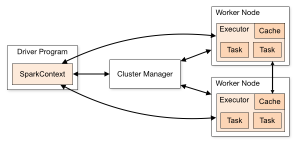 |
| Spark Driver | sends work we have 1 of those. |
| Spark Worker | like multiple of them, we want enough RAM memory connecting to hdfs |
| RDD | Think distributed collection with good api, immutable, fault tolerant |
#Partitions > #Executors |
* Optimize: At least many partitions (shard) to data like num of executors * So that each executor can work in parallel on some partition of the data |
| Immutability | FirstRDD points to SecondRDD points to ThirdRDD (transformations) |
| Fault Tolerance | If spark-worker fails work restarts on another spark-worker by spark-driver |
| Partitioning | Data is broken into partitions 3 |
| Worker node 1* Executor | |
| Transformations VS Actions | * Transformations [Lazy]: map, flatMap, filter, groupBy, mapValues, … * Actions: take, count, collect, reduce, top |
| Skeleton Project | |
| dependency | * “org.apache.spark” %% “spark-core” * create fatJar in assembly |
| Use Spark | |
| create SparkContext | * val sparkConf = new SparkConf().setAppName("somename").set("spark.io.compress.codec", "lzf") * val sc = new SparkContext(conf)* main standard java main method to run your code. |
| submit it | spark-submit com.mypackage.MySparkApp —master local[*] my-fat-jar-without-spark.jar // spark-submit is part of spark we downloaded // [*] use cpu cores as many as you have // To deploy to cluster you are going to have many more params |
| Spark API | |
spark-shell |
Explore the api with spark shell, already has spark context sc |
sc.makeRDD(List(1,2)) |
|
rdd.map |
val myRdd = rdd.map(_ * 2) // returns RDD |
myRdd.collect() |
Array(2,4) |
rdd.cache() |
So that if you have multiple .action() like .collect() data won’t be referched for the transformations rdd again. |
| Local dev | |
| Spark Dependency | |
| Main | object SparkExample extends App<br />override def main(args: Array[String]): Unit = { |
| Spark conf and context | val conf = new SparkConf().setAppName("parse my book").setMaster("local[*]")<br />val sc = new SparkContext(conf) |
| Load text from http | |
| Reduce by top words | |
| Performance | |
| *ByKey | reduceByKey much more efficient than reduce, no shuffle. *byKey. |
| Driver Node RAM | Result < RAM on driver machine, result returned through driver Otherwise out of memory. |
| minimize shuffles | The less you have the better spark will utilize data locallity and memory |
| Beginning NLP | |
| High dimentionality | text analytics is a high dimentionality problem, it’s not infrequent to have 100K features. |
| Topic | HOWTO |
|---|---|
| Study Resources | |
| General Big Data |  |
| Apache Spark |  |
| Amazon EMR | https://aws.amazon.com/emr/getting-started/ |
| Data Science RND Workflow | https://alexioannides.com/2016/08/16/building-a-data-science-platform-for-rd-part-1-setting-up-aws/ Zeppelin, AWS, Spark |
- AAS - Advanced Analytics with Spark
Which programming language is better R, Scala or Python?
I recently answered this question in quora, I didn’t phrase the question, but it’s a good starting point. I basically stay away from language debates as you will see, but this one really interested me. As I have debated with myself alot and was researching this specific question for myself, I basically wanted to know which one should I use for my next data project and here are my personal insights. (Please let me know what you think! :)
This is how I treat R, Scala, Python VS, which to choose saga. I basically use each for it’s better strength, here is the recipe. This is my personal view and usage of the languages.
Use R as a replacement for a spreadsheet **. Together with **RStudio it makes a killer statistics, plotting and data analytics application.
You can take log files, parse them, graph them, pivot table them, filter. And all with great support from RStudio - it’s a killer data analysis language and workspace, you should study as a replacement for spreadsheet workings.
Do you want to grep some lines from a text file no problem just use: dateLines <- grep(x = mylog, pattern = “^–”, value = TRUE). It’s a backfiring arrow, it’s both easy to write - once you know the command you need to use! - It’s many times very difficult to figure out what is the correct command to use, practice is the key, note taking is the key, you need time for that, consider do you have the time for that, if not just use it as your little spreadsheet and use it from time to time until you get better with it, save a note or doc with useful R command’s and you will find that with a few commands + few plotting commands you are a small king in it’s realm. This example of grep is only one of a million of crazy abilities and matrix manipulation and plotting and RStudio will have you doing analytics like crazy on data.
If you have no time for the above I still highly recommend you to install RStudio and use it from time to time, get the hang of it, there is nothing like it so far that I know that is so good for quick data analysis, quick statistics, just give it a shot and try to replace your routine calculations, quick data manipulations tasks with it.
You can also move on and do machine learning in R, it has extremely powerful libraries for that (rpart, caret, e1071, …) and by all means if you and your teams are fluent with it feel free to move on, but me personally would use it only for speculations and quick analysis or quick models, I stop there, it can be very quick but this is when I turn to language number 2 python.
Use Python for small to medium sized data processing applications. Python tough introduced some type checking in recent releases (which is awesome), is an interpreted language (just like R) but it’s a more of a standard programming language, as such you have the great benefit of speed of programming. You just write your code and run. However the caveat is that you don’t have the amazing compiler and features (the good ones not the kitchen sink one) from scala. Therefore as long as your project is small to medium sized.
It is going to be very helpful as you will utilize NLTK, matplotlib, numpy, pandas, and you will have great time and happy path learning and using them. This will take you on the fast route to machine learning, with great examples bundled in the libraries.
I’m not saying you cannot do it with R or scala with great success I’m saying as for my personal use this is the best most intuitive way to do that I use it for what’s it’s best.
I want quick analysis of csv I turn to R. I want a bulletproof fast app to scale in time I use scala. If my project is expected to be one big with many developers this is where I turn to language/framework number 3 - to java/scala.
Use scala(or java) for larger robust projects to ease maintenance. While many would argue that scala is bad for maintenance, I would argue that it’s not necessarily the case. java and scala with their mostly super strongly typed and compiled features, make them a great language for the large scale. You have spark opennlp libraries for your machine learning and big data. They are robust, they work in scale, it’s true it would take you longer time to code than in python but the maintenance and onboarding of new personal would be easier, at least in my cases.
Data is modeled with case classes.
Proper function signatures.
Proper immutability.
Proper separation of concerns.
While the above could be applied in any of the above languages it’s goes more naturally with scala/java.
But if you don’t have time or want to work with them all, then this is what I would do:
R - Research, plot, data analysis.
Python - small/medium scale project to build models and analyze data, fast startup or small team.
Scala/Java - Robust programming with many developers and teams, less machine learning utilities than python and R, but, it makes up by the increased code maintenance for multiple many developers teams.
It’s a challenge to learn them all and i’m still in this challenge, and it’s a true headache but at the end you benefit. If you want only one of them I would ask:
- Am I managing a project with many teams, many workers, speed is not the topmost priority, stability is the priority - java/scala.
- A few personal project I need quick results, I need quick machine learning on a startup - python.
- I just want to hack on my laptop data analysis and enhance my spreadsheet data analysis, machine learning skills - python or R